In my 7th semester in engineering i and my friends wanted to work on deep neural networks, we were interested mainly because we started working on a project which required knowledge about DNN’s like DBN( Deep Bayesian networks) , SAE/SDE ( Staked auto encoder’s) etc .
The project was basically to implement this paper. It was to predict traffic flow in a certain road/ highway .We learnt various techniques of neural network prediction out of which a Deep Belief Network aka Deep Bayesian network was one of my favorite.
Although the paper was based on a stacked auto encoders which i will be posting in my next blog , i wanted to experiment with DBN’s.
Here’s a little introduction about DBN’s ( Deep Belief Networks) from wiki:
In machine learning, a deep belief network (DBN) is a generative graphical model, or alternatively a type of deep neural network, composed of multiple layers of latent variables (“hidden units”), with connections between the layers but not between units within each layer.
When trained on a set of examples in an unsupervised way, a DBN can learn to probabilistically reconstruct its inputs. The layers then act as feature detectors on inputs. After this learning step, a DBN can be further trained in a supervised way to perform classification.
The Easiest way to work with your DBN and test it on a data is using Public data sets like MNIST . I have created my own DBN by learning from here. deeplearning.net is especially useful for beginners wanting to get their hands on deep neural network algorithms , i think it gives the best insights and is really well documented and for a beginner using their tutorials is one of the best way to get into the world of Deep Neural Networks. Scikitlearn is another such tutorial page that gives you detailed insight into algorithms and code alike.
For this particular experiment i used(requirement) :
pyprind is a good python tool that provides a progress bar and a percentage indicator object that let you track the progress of a loop structure or other iterative computation.This is especially useful when dealing with large data sets.
here’s the code of the program which uses CUDAmat to perform GPU calculations.
[code language="python"]
#coding: utf-8

from __future__ import division
import time
import numpy as np
import cudamat as cm
import pyprind

class RestrictedBoltzmanMachine(object):

 def __init__(self, n_hidden, learning_rate=0.1, momentum=0.9, n_epochs=30, batch_size=128, k=1, title=''):
 self.n_hidden = n_hidden
 self.learning_rate = learning_rate
 self.momentum = momentum
 self.n_epochs = n_epochs
 self.batch_size = batch_size
 self.k = k
 self.title = title

 def transform(self, v, h):
 """
 Parameters:
 v : the visible input activation
 h : the target to write the hidden activation
 """
 cm.dot(self.W.T, v, target = h)
 h.add_col_vec(self.hidden_bias)
 h.apply_sigmoid()

 def sample_hidden(self, v, h_mean, h):
 """
 Parameters:
 v : the visible input activation
 h_mean : the target to write the hidden activation
 h: the target to write the hidden sample
 """
 self.transform(v, h_mean)
 h.fill_with_rand()
 h.less_than(h_mean)

 def sample_visible(self, h, v_mean, v):
 """
 Parameters:
 h : the hidden activation
 v_mean : the target to write the visible activation
 v: the target to write the visible sample
 """
 self.reverse_transform(h, v_mean)
 v.fill_with_rand()
 v.less_than(v_mean)

 def reverse_transform(self, h, v):
 """
 Parameters:
 h : the hidden activation
 v : the target to write the visible activation
 """
 cm.dot(self.W, h, target = v)
 v.add_col_vec(self.visible_bias)
 v.apply_sigmoid()

 def fit(self, input, verbose=1):
 """
 Parameters
 ----------
 input : CUDAMatrix array, shape (n_components, n_samples) - opposite of scikit-learn
 """
 n_samples = input.shape[1]
 num_batches = n_samples // self.batch_size

 # model parameters
 self.n_visible = input.shape[0]

 # initialize weights
 self.W = cm.CUDAMatrix(0.1 * np.random.randn(self.n_visible, self.n_hidden))
 self.visible_bias = cm.CUDAMatrix(np.zeros((self.n_visible, 1)))
 self.hidden_bias = cm.CUDAMatrix(-4.*np.ones((self.n_hidden, 1)))

 # initialize weight updates
 u_W = cm.CUDAMatrix(np.zeros((self.n_visible , self.n_hidden )))
 u_visible_bias = cm.CUDAMatrix(np.zeros((self.n_visible , 1)))
 u_hidden_bias = cm.CUDAMatrix(np.zeros((self.n_hidden , 1)))

 # initialize temporary storage
 v = cm.empty((self.n_visible, self.batch_size))
 h = cm.empty((self.n_hidden , self.batch_size))
 r = cm.empty((self.n_hidden , self.batch_size))

 if verbose == 1:
 bar = pyprind.ProgBar(self.n_epochs, title=self.title)

 for epoch in range(self.n_epochs):
 start_time = time.time()
 err = []

 for batch in range(num_batches):
 # get current minibatch
 v_true = input.slice(batch*self.batch_size, (batch + 1)*self.batch_size)
 v.assign(v_true)

 # apply momentum
 u_W.mult(self.momentum)
 u_visible_bias.mult(self.momentum)
 u_hidden_bias.mult(self.momentum)

 # positive phase
 self.transform(v, h)

 u_W.add_dot(v, h.T)
 u_visible_bias.add_sums(v, axis = 1)
 u_hidden_bias.add_sums(h, axis = 1)

 # sample hiddens
 r.fill_with_rand()
 r.less_than(h, target = h)

 # negative phase CD-k
 for n in xrange(self.k):
 self.reverse_transform(h, v)
 self.transform(v, h)

 u_W.subtract_dot(v, h.T)
 u_visible_bias.add_sums(v , axis = 1, mult = -1.)
 u_hidden_bias.add_sums(h , axis = 1, mult = -1.)

 # update weights
 self.W.add_mult(u_W, self.learning_rate/self.batch_size)
 self.visible_bias.add_mult(u_visible_bias , self.learning_rate/self.batch_size)
 self.hidden_bias.add_mult(u_hidden_bias , self.learning_rate/self.batch_size)

 # calculate reconstruction error
 v.subtract(v_true)
 err.append(v.euclid_norm()**2 / (self.n_visible * self.batch_size))

 if verbose == 1:
 bar.update()
 elif verbose > 1:
 print("Epoch: %i, MSE: %.6f, Time: %.6f s" % (epoch+1, np.mean(err), (time.time() - start_time)))

 # frees memory
 u_W.free_device_memory()
 u_visible_bias.free_device_memory()
 u_hidden_bias.free_device_memory()
 v.free_device_memory()
 h.free_device_memory()
 r.free_device_memory()

class DeepBeliefNetwork(object):

 def __init__(self, layers):
 self.layers = layers

 def fit(self, input):
 """
 Train each layer of the network
 Parameters
 ----------
 input: A CUDAMatrix shaped as (n_features, n_samples)
 """
 n_samples = input.shape[1]

 for n, layer in enumerate(self.layers):
 layer.fit(input)

 if n+1 < len(self.layers):
 h = cm.empty((layer.n_hidden, n_samples))
 layer.transform(input, h)

 if n > 0:
 input.free_device_memory()

 input = h

 if len(self.layers) > 1:
 input.free_device_memory()

 def transform(self, input):
 """
 Transform the input through each layer
 Parameters
 ----------
 input: A CUDAMatrix shaped as the first layer
 Return
 ------
 A newly allocated CUDAMatrix with the shape of the last layer.
 """
 n_samples = input.shape[1]
 for n, layer in enumerate(layers):
 h = cm.empty((layer.n_hidden, n_samples))
 layer.transform(input, h)

 if n > 0:
 input.free_device_memory()

 input = h

 return input

 def reverse_transform(self, h):
 """
 Reverse transform from last to first layer
 Parameters
 ----------
 h: A CUDAMatrix shaped as the last layer
 Return
 ------
 A new CUDAMatrix with the shape of the first layer
 """
 for n, layer in enumerate(reversed(self.layers)):
 v = cm.empty(layer.visible_bias.shape)
 layer.reverse_transform(h, v)
 if n > 0:
 h.free_device_memory()
 h = v

 return v

 def dream(self, k=10):
 """
 Generate a pattern from this network.
 Return
 ------
 A new CUDAMatrix with the shape of the first layer
 """
 last_layer = self.layers[-1]

 v = cm.empty(last_layer.visible_bias.shape)
 h = cm.empty(last_layer.hidden_bias.shape)

 v_mean = cm.empty(last_layer.visible_bias.shape)
 h_mean = cm.empty(last_layer.hidden_bias.shape)

 h.fill_with_rand()
 for _ in xrange(k):
 last_layer.sample_visible(h, v_mean, v)
 last_layer.sample_hidden(v, h_mean, h)

 v.free_device_memory()
 v_mean.free_device_memory()
 h_mean.free_device_memory()

 return self.reverse_transform(h)
[/code]
Using Cuda as above enables dramatic increases in computing performance by harnessing the power of the graphics processing unit (GPU). With millions of CUDA-enabled GPUs sold to date, software developers, scientists and researchers are finding broad-ranging uses for GPU computing with CUDA.
Performance matters especially when processing large amounts of data ,withthe big data boom ,more and more people are preferring GPU computation .
Here’s how you can implement GPU processing on the DBN for MNIST.
#1 Initialize :
from __future__ import division

import numpy as np
from matplotlib import pyplot as plt
from rbm_cuda import RestrictedBoltzmanMachine, DeepBeliefNetwork
import cudamat as cm

%matplotlib inline

# Initialize CUDA
cm.cublas_init()
cm.CUDAMatrix.init_random(1)
#2 Load training data:
X = np.load("input/mnist.npy")

# Load data into GPU (it needs to be (n_features, n_samples) shape, so we save the transposition)
Xc = cm.CUDAMatrix(X.T)
#3 Create a DBN with layers of RBM ( in my example 6 RBM’s):
dbn = DeepBeliefNetwork([ RestrictedBoltzmanMachine(512, title="layer-1", n_epochs=50, batch_size=1000, momentum=.1),
                          RestrictedBoltzmanMachine(512, title="layer-2", n_epochs=50, batch_size=1000, momentum=.3),
                          RestrictedBoltzmanMachine(128, title="layer-3", n_epochs=50, batch_size=1000, momentum=.4),
                          RestrictedBoltzmanMachine(128, title="layer-4", n_epochs=50, batch_size=1000, momentum=.5),
                          RestrictedBoltzmanMachine(64 , title="layer-5", n_epochs=50, batch_size=1000, momentum=.6),
                          RestrictedBoltzmanMachine(64 , title="layer-6", n_epochs=50, batch_size=1000, momentum=.8),
                        ])
#4 Train the DBN with data :
layer-1
0%                          100%
[##############################] | ETA[sec]: 0.000
Total time elapsed: 9.801 sec
layer-2
0%                          100%
[##############################] | ETA[sec]: 0.000
Total time elapsed: 6.510 sec
layer-3
0%                          100%
[##############################] | ETA[sec]: 0.000
Total time elapsed: 2.803 sec
layer-4
0%                          100%
[##############################] | ETA[sec]: 0.000
Total time elapsed: 1.860 sec
layer-5
0%                          100%
[##############################] | ETA[sec]: 0.000
Total time elapsed: 1.607 sec
layer-6
0%                          100%
[##############################] | ETA[sec]: 0.000
Total time elapsed: 1.418 sec
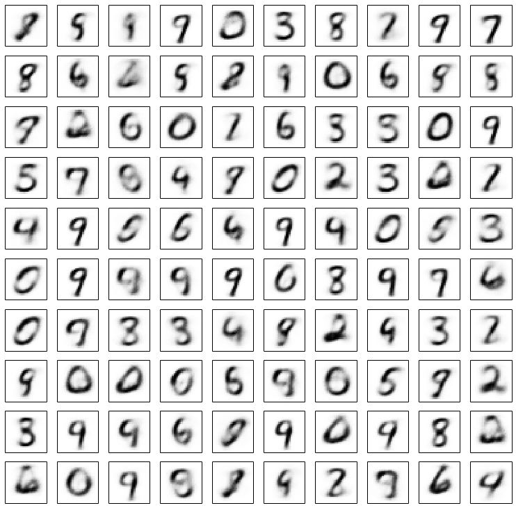
#5 Plot the generated data from the network :
plt.figure(figsize=(12.2, 12))
for i in xrange(100):
    plt.subplot(10, 10, i + 1)
    plt.imshow(dbn.dream(k=50).asarray().reshape((28, 28)), cmap=plt.cm.gray_r,
               interpolation='nearest')
    plt.xticks(())
    plt.yticks(())
plt.subplots_adjust(0.08, 0.02, 0.92, 0.85, 0.08, 0.23)
plt.show()
#6 shut down cuda :
# shutdown CUDA
cm.cublas_shutdown()
Hope this post helps someone , feel free to experiment it yourself and let me know if you come across any errors or have any questions
“CARPE DIEM ”
You can follow me on GITHUB !!!